A Ramble Through the Cluster Data, Part 2: Quantifying and Visualising Clusters.

In part 1, I introduced you to the cluster data set, a second passim data set that is slightly different from the pairwise data set that the KITAB team use in their daily research. The cluster data set brings together the pairwise alignments that overlap by more than 80% into larger clusters containing multiple book milestones. These clusters can be used to explore stemmatic relationships between texts, or may even reveal how a set of texts rely on the same lost source text. I will be using this data set in my research for the ERC team’s forthcoming volume. However, before I engage in a closer study of individual clusters and their historical importance (I will begin to explore this in part 3), it is important to understand the nature of single-link clustering and its limitations and to explore the scale of the cluster data set in general. This will guide me in identifying clusters of interest and help to contextualise my findings later on.

Understanding the scale of the clusters: single-link clustering and the pre-modern Arabic tradition

In the example in part 1 we moved from one pairwise alignment to a cluster of alignments. So far so simple. However, the difficulty comes with identifying relevant and useful clusters within the data set. The cluster dataset is enormous. There are three and a half million clusters. The smallest clusters are size 2 – these are the most common. The largest cluster (cluster number 1) contains 903302 milestones (found in 4960 books). That means that it contains multiple milestones from nearly every book in the corpus. If one studies the text of cluster 1, one will find that a lot of it appears unrelated. This is a weakness in single-link clustering. As a single-link with any other text fragment in the cluster is needed (that is, shared text above a threshold of 80%) to pull another alignment into a cluster and with the addition of each alignment new text is added, alignments added at the end of the cluster can be very different to those added at the start.

For ease of explanation, let us discuss an example in English. Consider these four alignments that each overlap by more than 50%:

1. The quick brown fox jumps over the lazy dog

2. In the very famous phrase, "The quick brown fox jumps..."

3. In the very famous phrase, "The eagle has left the building"

4. The phrase "The eagle has left the building" was originally used to disband crowds

Alignment 1 does not have anything in common with alignments 3 and 4.¹

For an example from the real cluster data, see figure 1. This gives a sample of pairwise alignments that belong to a cluster containing 15 milestones in total - I have only provided a sampling of the milestones, enough to illustrate how the cluster is linked together. Small but important similarities have led strong instances of text reuse to be clustered with much weaker alignments. The final table in the series shows how the last alignment in the sequence of the cluster is entirely unrelated to the first, apart from a few quite vague words. The pair of milestones 605 and 9310 illustrate how a weak link has led to other alignments being added to the cluster. There is strong text reuse between 605 and 9732, and between 9310 and 634. By comparison, 605 and 9310 are linked on the basis the phrase ‘Ibn Hibban said in the Majruhin’ and on a shared citation of a text (the footnotes have yet to be removed from these two OpenITI texts).² Thus in this case three strong clusters of texts have been drawn into one cluster by these weaker links. From this example it is easy to see how similarities in chains of transmission (isnads) in particular could lead to the creation of enormous clusters.

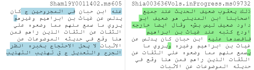
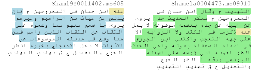
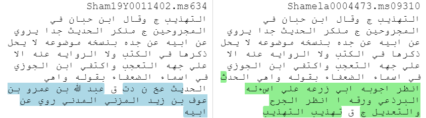
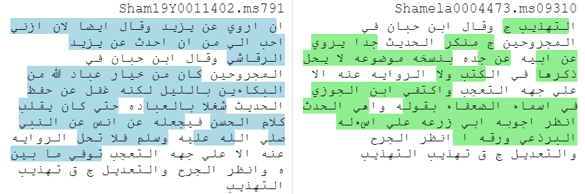
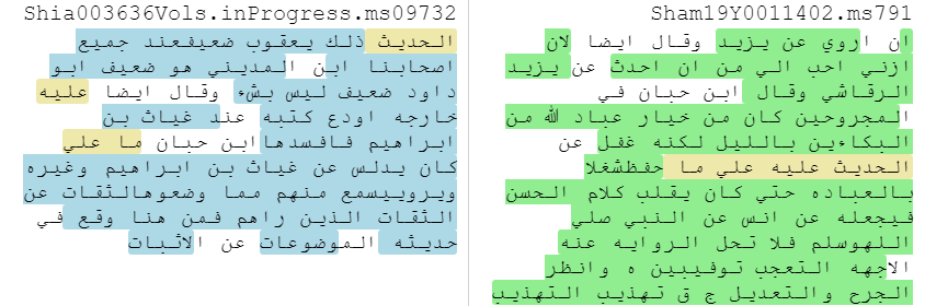
Figure 1: A selection of pairwise alignments from cluster 34359801867, which contains 15 book milestones in total, given as a series of tables. Each table in the series contains a milestone from the table above (for example, the second table contains ms605, which is also in the first table), and so they each represent a step in the creation of the cluster. This representation is somewhat artificial and it has been reconstructed after the fact, as passim’s output does not indicate the manner in which each cluster has been formed. These tables were produced using the diff viewer developed by Peter Verkinderen.

Lay of the land: some visualisations and statistics

Even if we exclude extremely large clusters (for example, exclude all clusters that contain more than 500 milestones), the data set is still too large to be understood through one visualisation. Figure 2 gives an example of a graph drawn from the cluster data for books written before 900/1494. Each node (a dot) is an author in the corpus and each edge (that is, the line connecting two nodes) represents a cluster shared between two authors (using authors rather than books reduces the total number of nodes). Edges are weighted based on the number of clusters shared between two authors. To help distinguish the nodes, they have been coloured according to the author’s death date (darker nodes are later).

Figure 2: A graph of all authors in the corpus written who died before 900/1494 with edges weighted according to the number of clusters shared between authors.

Even though figure 2 has been drawn taking account of edge weight (that is, broadly, edges with lower weights are closer to the outside of the graph), it is impossible to derive any meaning from this graph. This is because nearly all of our authors are connected in some way by a cluster. In reality most connections are only very small (the median edge weight is 2 and the mode is 1), but some authors are very connected (the mean edge weight is 22 – so very large edge weights are pushing up the average).³

The largest edge in this graph is shared between Ibn ʿAskakir and Ibn Manzur al-Ifriqi, with 31855 clusters shared between these authors. This is not surprising as Ibn Manzur abbreviated Ibn ʿAsakir’s Taʾrikh Madinat Dimashq, which is the largest pre-modern book in the corpus (lots of aligned milestones equals lots of clusters). However, even if we exclude all clusters with a weight of 2 from the count (that is, we exclude all clusters that represent only text reuse between these two texts), the cluster count is still 22219. This shows how Ibn ʿAsakir had himself reused material for his work, which might in turn have been reused by others.

In short, many pre-modern authors in the OpenITI corpus are connected by at least one cluster and a smaller number are connected by a significant number of clusters. Next, we should ask how large the clusters are. As noted above, the vast majority of clusters contain two books (that is, they represent only pairwise relationships). However, there is still a large number of clusters that contain 3 or more book milestones.

Figure 3 gives a histogram for the entirety of the cluster dataset, plotting the frequency of clusters according to their size. As can be seen in this figure , larger clusters are much less frequent in the dataset, but they do occur. There are two huge outliers (a cluster of 903,302 milestones and another of 2874). There are, however, a number of clusters that contain over 500 book milestones. It is very likely that these clusters are not meaningfully related, a consequence of the single-link clustering described above, but they would need closer investigation.

Figure 3: A histogram showing the frequencies of clusters at different sizes. In order to make the bars readable, both the x and y axis use log scales (the gaps between the values get larger the further along the axis you proceed). As a result, you should pay careful attention to the values on each axis when reading this graph.

We can be more certain that clusters that contain fewer than 20 milestones are more meaningfully related (although as the example in figure 1 above showed, even smaller clusters can become unrelated). Figure 4 graphs the frequencies of clusters by their size, up to size 20, and provides an additional bar for all those clusters that contain more than 20 milestones. Table 1 gives the frequencies and their percentage of the total data set.

Figure 4: A barchart of the frequencies of clusters by their size (focussing on clusters that contain up to 20 book milestones, with all clusters above size 20 given in the final bar). In order to make the bars visible, a logarithmic scale has been used for the count on the y axis. For the values see table 4.

Cluster Size	Count	Percentage
2	2,321,187	65.74
3	636,594	18.03
4	246,287	6.98
5	118,034	3.34
6	64,988	1.84
7	39,142	1.11
8	25,542	0.72
9	17,258	0.49
10	12,201	0.35
11	8,996	0.25
12	6,808	0.19
13	5,245	0.15
14	4,138	0.12
15	3,215	0.09
16	2,625	0.07
17	2,173	0.06
18	1,866	0.05
19	1,600	0.05
20	1,241	0.04
>20	11,621	0.33
Total clusters	3,530,761	100

Table 1: Frequencies of clusters of each size, and the percentage of the dataset that they represent.

As a percentage of the total dataset, clusters of 3 and bigger appear to be quite small, but in terms of absolute counts there are still a large number of clusters containing between 3 and 10 book milestones. It is clusters of this size that can be most fruitful for the study of historiography and its transmission and for comparing different accounts of the same event.

The next waypoint

In this blog post it was my aim to explore single-link clustering, its shortfalls and to analyse the scale of the cluster data set. Very large clusters appear to not be meaningfully related and the majority of the clusters are between 2 and 10 book milestones in size. Clusters of this size still contain a large number of book milestones and they, moreover, cover a variety of subjects – far beyond the historiography that I wish to study. The next blog post will, therefore, concern my attempts to search the clusters and identify those of interest to my research.

1. I am grateful to Peter Verkinderen for suggesting this example, which helps greatly to clarify the problem. ↩

2. An example like this potentially illustrates the importance of cleaning OpenITI texts for this kind of analysis. Removing modern footnotes which contain repetitive phrasing and can cite similar books will help passim to build less noisy clusters. ↩

3. To clarify: these are different ways of calculating an average from the data. Median is the middle point of the data, when the values are ordered according to size. Mode is the value that appears most in the data set. The mean is the value that we typically think of when we speak of averages (calculated by adding all the values together and dividing that by the number of data points). To give an example: here is a list of 11 data points: ‘2, 4, 4, 4, 9, 9, 9, 9, 9, 9, 9’. In this data set, the median is 9 (the sixth data point in the list), the mode is 9 and the mean is 6.2. Notice how the median and mode take better account of the values that are more present in the data set, where the mean is lower because there are some very small (albeit less frequent) values in the data set. As infrequent but very large or very small values can bias the mean, it is not always the best way to take an average of a data set. ↩